Introduction
If you've used any AI image generator in the last two years — Midjourney, DALL-E, Stable Diffusion — you've used a diffusion model. These models are behind nearly every recent breakthrough in AI-generated visuals, from photorealistic portraits to fantastical landscapes that never existed.
The name "diffusion" comes from physics. Think of a drop of ink falling into a glass of water: it spreads outward, mixing until the water is uniformly tinted. That physical process is diffusion. The AI version takes the same idea but runs it in reverse — starting from the uniformly mixed state and reconstructing the original drop.
That sounds like it should be impossibly hard. But the core mechanism is surprisingly elegant. By the end of this article, you'll understand the fundamental idea behind every diffusion model, and you'll see that it's simpler than most explanations make it seem. No PhD required.
The Forward Process: Adding Noise
Let's start with something concrete. Take a photograph — say, a picture of a cat. It's a grid of pixels, each with a specific color value. Now add a tiny amount of random noise to every pixel. Noise here just means small random changes: bump some pixels slightly brighter, others slightly darker, following a bell curve distribution (called Gaussian noise).
After one round of noise, the image looks almost identical. Maybe you'd notice a faint grain if you zoomed in. Now do it again. And again. Each time, the image gets a little fuzzier, a little less recognizable. After hundreds of steps, the cat is completely gone. All you have left is pure static — the visual equivalent of white noise on an untuned television.
This systematic destruction is called the forward process. It takes a clean image and gradually corrupts it into random noise over many steps (typically around 1,000 in the original formulation).
Here's an analogy that makes this click. Imagine pouring a drop of ink into a glass of still water. At first, you can see the ink as a distinct blob. Over time, it spreads and mixes. Eventually, the water is a uniform pale color and you can't tell where the ink was originally dropped. The information about the starting position has been destroyed — diffused away.
The crucial detail is that the math at each step is dead simple. You're just adding a sample from a Gaussian distribution with a known variance. And because you control the process, you know exactly how much noise was added at each step. This is not random destruction — it's carefully calibrated destruction with a full paper trail. That paper trail is what makes the reverse process possible.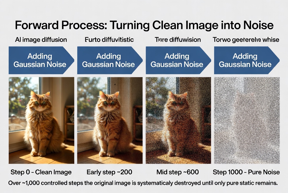 The forward process: a clean image is gradually destroyed by adding Gaussian noise at each step, until only pure static remains.
The Reverse Process: Learning to Denoise
Here's where the magic happens. What if you could run this whole process backward? Start with pure noise and, step by step, remove the noise to reveal a clean image?
That's exactly what a diffusion model learns to do. You train a neural network — specifically, a type called a U-Net — on a simple task: given a noisy image, predict what the noise looks like. Not the clean image. Just the noise. This is a subtle but important distinction.
During training, you take millions of real images, add known amounts of noise to them (using the forward process), and then ask the network: "Here's a noisy image at step 400. What does the noise component look like?" The network learns to separate signal from noise at every corruption level.
At generation time, you start with a sample of pure random noise and feed it to the trained network. The network predicts the noise component. You subtract that prediction from the input, and you get something slightly less noisy. Feed that result back in. Subtract again. Repeat for hundreds of steps. Gradually, structure emerges from the static — edges form, shapes coalesce, details sharpen — until you have a clean, coherent image.
The network itself never "imagines" or "creates" in any direct sense. It has learned one narrow skill extremely well: recognizing what noise looks like and separating it from real content. The generation of an image is an emergent consequence of applying that skill repeatedly.
A good analogy: imagine a photo restoration expert who has examined millions of damaged photographs. Show them a photo with water stains, and they can tell you exactly which marks are damage and which are part of the original picture. They're not painting a new photo — they're stripping away corruption. A diffusion model does essentially the same thing, except the "damage" is synthetic Gaussian noise, and the "expert" is a neural network with billions of parameters.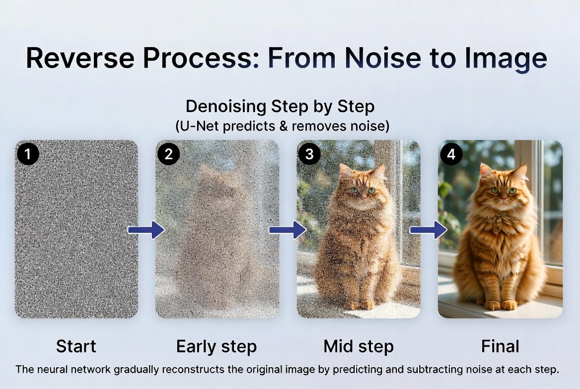 The reverse process: the same neural network is applied at each step, predicting and removing noise to gradually reveal a coherent image.
How Text Prompts Steer Generation
So far we have a process that goes from noise to images. But there's a problem: you can't control what image comes out. Without guidance, the model just produces random images from its training distribution. To make this useful, we need a steering mechanism.
The solution is elegant. During training, each image is paired with a text description. The neural network receives two inputs at each denoising step: the current noisy image and a text embedding (a numerical representation of the prompt, produced by a separate text encoder like CLIP). The text acts as a compass — it doesn't determine every pixel, but it points the denoising process in a semantic direction.
The same starting noise, denoised with the prompt "a tabby cat sitting on a windowsill," will produce something entirely different from the same noise denoised with "a snow-capped mountain at sunset." The noise is the raw material; the text prompt is the blueprint. This mechanism is called conditioning — the text conditions the generation process.
In practice, modern models use a technique called classifier-free guidance to make this work well. At each denoising step, the model actually runs twice: once with the text prompt and once without it. It then compares the two predictions and amplifies the difference. The "guidance scale" parameter you see in tools like Stable Diffusion controls how aggressively this amplification is applied. High guidance scale means the output adheres more closely to your prompt but may look less natural. Low guidance scale gives more creative latitude but may drift from your intent.
This two-pass approach is why generation isn't quite twice as fast as you'd expect — and it's also why the quality is so much better than earlier conditioning methods. The model learns the difference between "what I'd generate anyway" and "what I'd generate given this specific instruction," and leans into that difference.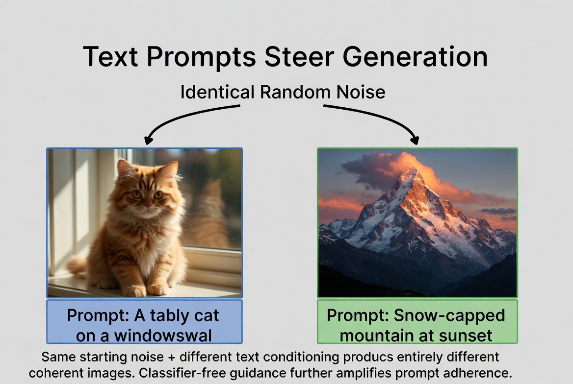 Text conditioning: identical starting noise produces entirely different images depending on the text prompt used to guide denoising.
Making It Practical: Fewer Steps
There's a practical problem with what we've described so far. The original DDPM (Denoising Diffusion Probabilistic Model) paper used 1,000 denoising steps to generate a single image. Each step requires a full forward pass through a large neural network. On a modern GPU, that could take several minutes per image. For a consumer product, that's a non-starter.
The first major breakthrough was DDIM (Denoising Diffusion Implicit Models). The insight was that you don't have to visit every single noise level during generation. You can skip steps — jumping from step 1,000 to step 950, then to step 900 — while still producing good results. Think of it like an express train that skips local stops: you get to the same destination much faster. DDIM reduced generation to 50-100 steps with minimal quality loss.
Then came distillation. The idea is straightforward: train a smaller "student" model to mimic what the larger "teacher" model does in many steps, but do it in far fewer steps. Essentially, the student learns to take bigger jumps through the denoising trajectory. Progressive distillation halved the step count repeatedly — from 1,000 to 500, then 250, then 125, down to as few as 4 steps.
More recent approaches like consistency models and flow matching have pushed this even further, enabling single-step or two-step generation with quality that would have been state-of-the-art just a year or two earlier. This is why modern tools like Stable Diffusion XL and DALL-E 3 can generate images in seconds rather than minutes.
The speed improvement wasn't just a nice optimization — it was the difference between a research curiosity and a product that millions of people use. Without these acceleration techniques, real-time creative tools built on diffusion models simply wouldn't exist.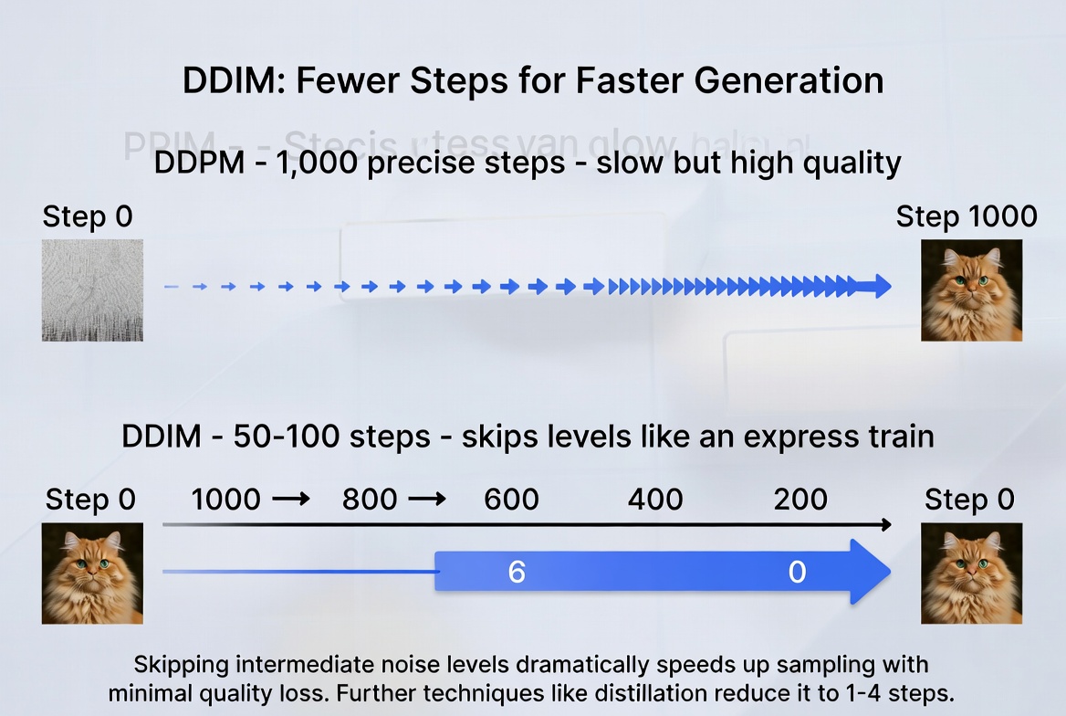 Fewer denoising steps, faster generation: techniques like DDIM and distillation let models skip steps without significant quality loss.
Why Diffusion Won
Before diffusion models took over, the dominant approach for AI image generation was GANs — Generative Adversarial Networks. GANs work by pitting two neural networks against each other: a generator that creates images and a discriminator that tries to tell real from fake. The generator gets better at fooling the discriminator, and the discriminator gets better at catching fakes. In theory, this arms race produces incredibly realistic images.
In practice, GANs were nightmarish to train. The two networks had to stay in a delicate equilibrium. If the discriminator got too good too fast, the generator couldn't learn. If the generator found a way to exploit a weakness in the discriminator, it would produce only a narrow range of outputs — a failure mode called mode collapse. You might ask for diverse face images and get the same three faces over and over. Training was unstable, finicky, and required extensive hyperparameter tuning.
Diffusion models sidestepped all of this by having a radically simpler training objective: predict the noise in a noisy image. This is just regression — arguably the most well-understood problem in all of machine learning. There's no adversarial dynamic, no equilibrium to maintain, no mode collapse. You show the network a noisy image, it predicts the noise, you compute the error, and you update the weights. Training is stable and predictable.
The result was dramatic. Diffusion models produced more diverse outputs (no mode collapse), higher-quality details (especially in complex compositions), and were far more consistent to train. Within about two years of the key papers (Ho et al. 2020, Dhariwal & Nichol 2021), diffusion models had comprehensively replaced GANs as the state of the art for image generation. It wasn't even close.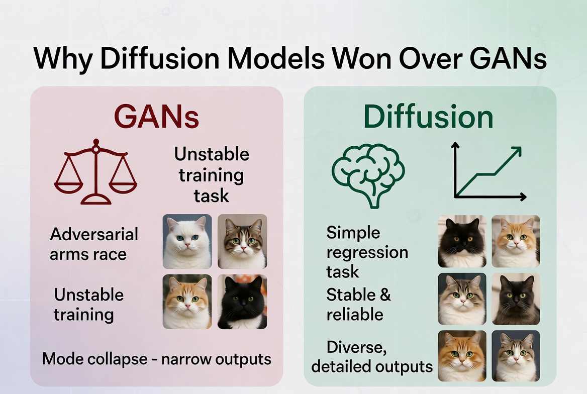 Why diffusion won: GANs required a delicate adversarial balance and suffered mode collapse, while diffusion models train stably with a simple denoising objective.
What This Means for Image-to-Video
You now understand the engine that powers AI image generation: learn to remove noise, and you can create images from nothing. The forward process destroys. The reverse process creates. Text conditioning steers. And clever scheduling makes it fast.
This same core idea — learn to denoise — also powers image-to-video models. Instead of generating a single image from noise, you generate a sequence of frames. But video adds a critical dimension: time. It's not enough for each individual frame to look good. The frames have to flow together smoothly, maintaining consistent objects, lighting, and motion from one frame to the next.
But there's one more concept we need to cover first: latent space. Running diffusion on raw pixels is computationally brutal. Modern models cheat — in a good way — by compressing images before applying the diffusion process. Understanding this compression trick is essential for understanding how any practical diffusion system works, from Stable Diffusion to video generation.