Introduction
Diffusion models generate amazing images, but there is a problem: they are incredibly slow when working with actual pixels. In the previous article, we saw how diffusion gradually removes noise to create images. What we glossed over is just how much data the model has to chew through at every single step.
A 512x512 image has 786,432 values (3 color channels times 512 times 512). Running the full diffusion process on that many numbers is computationally brutal. It works, but it is painfully slow.
The solution turns out to be surprisingly elegant: don't work with pixels at all. Instead, work with a compressed version of the image. This compressed space is called latent space, and understanding it is the key to understanding why modern AI image generation is practical enough to run on your laptop.
The Pixel Problem
Let's walk through the math to see why pixel-space diffusion hits a wall so quickly.
A standard 512x512 RGB image is a grid of pixels, each with three values (red, green, blue). That gives us 512 × 512 × 3 = 786,432 numbers. At every step of the diffusion process, the neural network has to process all of these numbers, compute how to adjust them, and output 786,432 updated values.
A typical diffusion process runs for around 50 steps. So during a single image generation, the network processes roughly 39 million values. And that is just for one 512x512 image. Want 1024x1024? Quadruple everything.
The early diffusion models, like the DDPM paper from 2020, worked directly in this pixel space. They produced beautiful results, but they could only handle small images (typically 256x256), and generation took minutes per image even on high-end GPUs. Training took weeks.
This was a dead end for practical applications. You cannot build a product that people actually use if every image takes five minutes to generate. The math was right, the results were gorgeous, but the approach did not scale. Something had to change.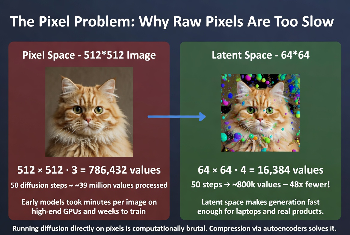 Running diffusion directly on pixels is computationally brutal. Compression via autoencoders solves it.
Autoencoders: Compress and Decompress
The key insight came from a different corner of machine learning: autoencoders. An autoencoder is a neural network built in two halves that learns to compress and decompress data.
The first half is the encoder. It takes a full-size image and squeezes it down into a much smaller representation. Think of it as the network learning what information is truly essential and throwing away the rest.
The second half is the decoder. It takes that small representation and reconstructs the original image from it. If the autoencoder is well-trained, the reconstructed image looks nearly identical to the original.
The small representation in the middle is called the latent representation, or simply the latent. This is where the name latent space comes from: the space of all possible compressed representations.
Here is an analogy. Imagine summarizing a 300-page novel into a 5-page synopsis. A good summary captures the essence of the story (characters, plot, themes) in far fewer words. You lose some nuance, but the core is preserved. The encoder writes the summary. The decoder expands it back into a full narrative.
Another way to think about it: it is like a zip file for images, but smarter. A zip file uses generic compression. An autoencoder has been trained on millions of images and has learned specifically what matters visually. It knows that smooth gradients can be described compactly, that edges carry more information than flat regions, and that certain textures follow predictable patterns.
In practice, the encoder compresses a 512x512 image down to a 64x64 representation. That is a 64x reduction in spatial size.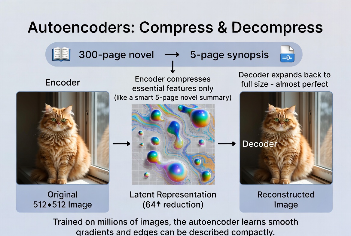 The autoencoder compresses a full-size image into a compact latent representation, then reconstructs it.
What Latent Space Actually Looks Like
So the latent is smaller, but what actually is it? It is not a tiny image. It is not pixels. It is a set of abstract features that the network has learned to extract.
The easiest way to think about latent space is as a map. Imagine a vast 2D plane where every point corresponds to an image. Images that look similar are placed near each other. All the cat photos cluster together in one region. Dog photos in another. Landscapes off to one side.
Here is where it gets interesting: the directions in this space are meaningful. Move in one direction and hair gets longer. Move in another and a face starts smiling. Move diagonally and you might get a smiling person with longer hair. The network has learned to organize visual concepts so that proximity means similarity.
This is why latent space interpolation works so well. If you pick two points in latent space (say, a cat and a dog) and smoothly walk between them, every point along the way also corresponds to a valid, plausible image. You get a seamless morph from cat to dog, passing through strange but coherent cat-dog hybrids.
Think of it like a periodic table for visual concepts. Just as the periodic table organizes elements so that neighbors share properties, latent space organizes images so that neighbors share visual features. Every position in the space corresponds to something meaningful, and there are no gaps or dead zones.
In reality, the latent space has far more than two dimensions (typically hundreds or thousands). But the principle is the same: it is a smooth, continuous space where proximity equals visual similarity.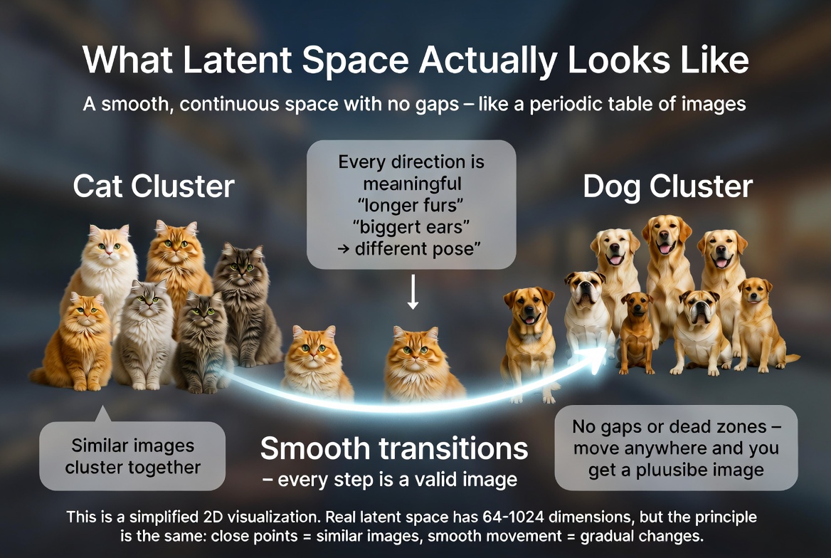 Latent space as a conceptual 2D map. Similar images cluster together, and the path between clusters produces smooth transitions.
Latent Diffusion: The Breakthrough
Now we can put the two ideas together. Instead of running the diffusion process on the full 512x512 pixel image, run it on the 64x64 latent. This is the core idea behind latent diffusion, and it changed everything.
The process works in three steps:
Step 1: Encode
If you are doing image-to-image generation (or image-to-video), the input image is first fed through the encoder to produce its latent representation. If you are generating from scratch, you simply start with random noise in the latent space. Either way, you begin with a small 64x64 tensor.
Step 2: Diffuse in latent space
The entire diffusion process (adding noise, then iteratively denoising) happens in this compact latent space. The neural network that does the denoising (typically a U-Net) only ever sees 64x64 inputs, never the full-resolution image. Every forward pass is fast because the data is small.
Step 3: Decode
Once diffusion is complete and you have a clean latent, the decoder expands it back to a full-resolution 512x512 image. This decoding step happens once, at the very end.
Let's look at the math. The latent representation is 64 × 64 × 4 channels = 16,384 values. The original pixel image is 512 × 512 × 3 channels = 786,432 values. That is a 48x reduction in the amount of data the diffusion model has to process at every step.
This is why Stable Diffusion can generate images in seconds on a consumer GPU. It is not that the GPU is magically fast. It is that the model is working in a space that is 48 times smaller than the actual image. The heavy lifting (compression and decompression) is done by the autoencoder, which only runs once at the beginning and once at the end.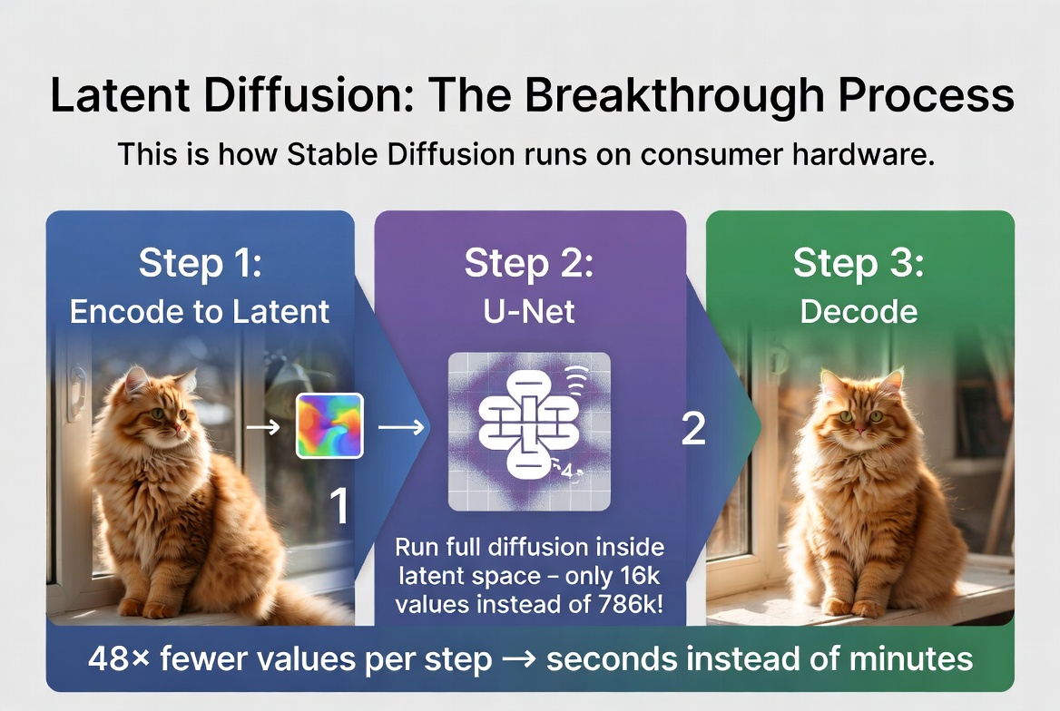 Latent diffusion: encode, diffuse in compressed space, decode. 48x fewer values per step means seconds instead of minutes.
VAE: The Specific Autoencoder
The particular type of autoencoder used in latent diffusion models is called a VAE, which stands for Variational Autoencoder. It is a specific flavor of autoencoder with one important twist.
A regular autoencoder encodes an image to a single fixed point in latent space. A VAE encodes it to a probability distribution instead. Think of it as encoding to a small fuzzy cloud rather than a precise pinpoint. During training, the decoder has to reconstruct the image from a random sample drawn from that cloud.
Why does this matter? Because it forces the latent space to be smooth and continuous. If the encoder mapped every image to an exact point with empty gaps between them, the diffusion process would constantly stumble into those gaps and produce garbage. The VAE's probabilistic encoding fills in those gaps, ensuring that every point in the latent space corresponds to a plausible image.
You do not need to understand the math behind the VAE to grasp latent diffusion. Just remember: VAE = the compression engine, and its special probabilistic design is what makes the latent space smooth enough for diffusion to work well in it.
Why This Changed Everything
Before latent diffusion arrived in 2022, diffusion models were an academic curiosity. The images they produced were stunning, but the computational requirements made them impractical for real-world use. You needed a top-tier GPU and several minutes to generate a single image.
The paper that changed this was "High-Resolution Image Synthesis with Latent Diffusion Models" by Robin Rombach, Andreas Blattmann, Dominik Lorenz, Patrick Esser, and Bjorn Ommer, published in 2022. It is one of the most impactful machine learning papers of the decade, and the basis for Stable Diffusion.
The concrete impact was staggering:
Training time dropped from weeks to days. Because the model operates on 48x less data at each step, you can train on the same hardware in a fraction of the time, or achieve better results in the same time.
Inference speed went from minutes to seconds. A consumer GPU with 8GB of VRAM could suddenly generate 512x512 images in under 10 seconds. This made real-time creative workflows possible for the first time.
Image resolution jumped from 256x256 (the practical limit of pixel-space diffusion) to 512x512 and beyond. Today, latent diffusion models routinely produce 1024x1024 images, something that would have been unthinkable with pixel-space approaches.
And the same compression trick scales to video. Instead of compressing 2D images into 2D latents, you can compress 3D video volumes (width, height, time) into compact 3D latent representations. This is what makes AI video generation possible on current hardware, which we will explore in the next article.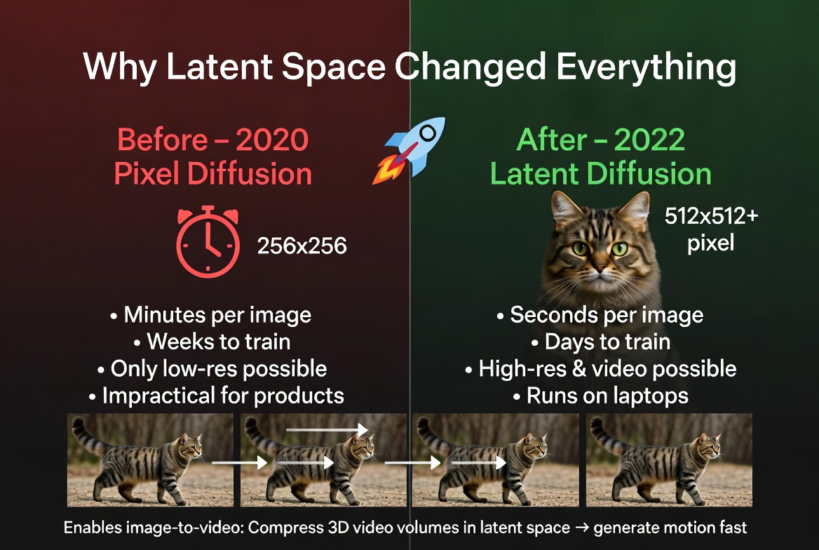 Before and after latent diffusion: from a research curiosity to a technology that runs on consumer hardware and enables video generation.
What This Means for Image-to-Video
When you upload a photo to a tool like picto.video, the very first thing that happens is encoding it into latent space. Your full-resolution image gets compressed down to a compact representation that captures its essential visual features.
From there, the AI model works entirely in this compressed space to generate motion. It figures out how objects should move, how lighting should change, how new frames should relate to each other, all at a fraction of the computational cost of working with raw pixels.
Once the model has generated the full sequence of latents (one for each frame), the decoder expands each one back to a full-resolution image, producing the final video.
This is why video generation is even possible on current hardware. A single frame at 512x512 is 786,432 values. A 4-second video at 24 frames per second is 96 frames, which adds up to 75 million pixel values. Without latent space compression, generating that would take hours. With it, it takes seconds to minutes.
In the next article, we will look at how image-to-video models extend diffusion into the time dimension, adding temporal layers that keep motion smooth and consistent across frames.